Tutorial

This notebook demonstrates the basic capabilities of the Empirical Redox Model.

*To run this code interactively in your web browser, click the “Launch Binder” button below:* (Note that the file may take a long time to load, and outputs will not be saved.)

Installing and Importing

The first step towards running the model is to ensure that all necessary packages are installed. If you are running in an interactive MyBinder instance, this has been done for you. If you are running the code locally, please ensure you have followed the installation steps: [COMING SOON]

Once you have installed the Empirical Redox Model package, you will need to import its modules into your script:

NOTE: To run a cell, click inside the shell and hit Shift+Enter. All cells in a notebook can be run from the top “Run” menu (“Run All Cells”)

NOTE: You may get some Deprecation Warnings when you import these modules. That’s fine!

# ---------------------------------------------------------------------------------------------------------------------
# Package Imports: These modules contain the functions and classes necessary for running the model.
# ---------------------------------------------------------------------------------------------------------------------

from empirical_redox_model import data_structures as data_struct
from empirical_redox_model import input_composition as input_comp
from empirical_redox_model import main

# ---------------------------------------------------------------------------------------------------------------------
# General Imports: It's also useful to have a few common packages imported into the code.
# ---------------------------------------------------------------------------------------------------------------------

import numpy as np
import matplotlib.pyplot as plt
import pandas as pd

# Suppress deprecation warnings in Binder script
import warnings
warnings.filterwarnings("ignore", category=DeprecationWarning)

Minimum Working Example

This code block demonstrates the minimum amount of code needed to run the Empirical Redox Model. Then, the code below breaks down the inputs and parameters, demonstrating how to use the model and adapt it to your own use case.

pot_TC = 1350
initial_assemblage = input_comp.get_WH05_starting_comp(bulk_Fe2O3=0.3)
initial_assemblage_in_garnet_field = input_comp.garnet_project(initial_assemblage, pot_TC, 4.0, spl_final=0.05, display=False)
model_run = main.ModelRun(
            label = 'Tp = 1350°C',
            potential_temperature_C = pot_TC,
            initial_assemblage = initial_assemblage_in_garnet_field,
        )
model_run.plot()

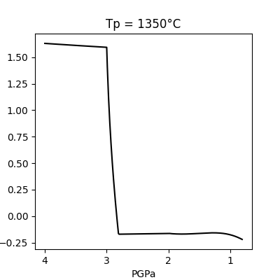
Tp = 1350°C : Successful run!

Breaking Down the Code

1. Determining Starting Composition

1a. Using Workman and Hart (2005) starting composition.

Currently, the only ‘built-in’ input composition is that of DMM from Workman and Hart (2005). You can access this composition using the following code (change the bulk_Fe2O3 value to your preferred value, if necessary):

initial_assemblage = input_comp.get_WH05_starting_comp(bulk_Fe2O3=0.3, display=False)

1b. Creating your own input composition.

If you wish to use a different starting composition, you can! It just takes a few more steps, but it’s also useful for understanding what the code is doing.

Example of how to format an input composition. Change these values as needed.

phase_modes = {'olv':57, 'opx':28, 'cpx':13, 'spl':2,
               'gt':0, 'liq':0, 'agg_liq':0}

phase_oxides = {
    # Minerals present in starting composition
    'olv':     {'SiO2':40.7,  'Al2O3':0,     'Fe2O3':0, 'FeO':10.16, 'MgO':48.59, 'CaO':0.05,  'Cr2O3':0},
    'opx':     {'SiO2':53.36, 'Al2O3':6.46,  'Fe2O3':0, 'FeO':6.27,  'MgO':30.55, 'CaO':2.18,  'Cr2O3':0.76},
    'cpx':     {'SiO2':50.61, 'Al2O3':7.87,  'Fe2O3':0, 'FeO':2.94,  'MgO':16.19, 'CaO':19.52, 'Cr2O3':1.20},
    'spl':     {'SiO2':0,     'Al2O3':57.54, 'Fe2O3':0, 'FeO':12.56, 'MgO':19.27, 'CaO':0,     'Cr2O3':10.23},
    # Minerals not present in starting composition
    'gt':      {'SiO2':0,     'Al2O3':0,     'Fe2O3':0, 'FeO':0,     'MgO':0,     'CaO':0,     'Cr2O3':0},
    'liq':     {'SiO2':0,     'Al2O3':0,     'Fe2O3':0, 'FeO':0,     'MgO':0,     'CaO':0,     'Cr2O3':0},
    'agg_liq': {'SiO2':0,     'Al2O3':0,     'Fe2O3':0, 'FeO':0,     'MgO':0,     'CaO':0,     'Cr2O3':0}
    }

Once you have your phase modes and phase oxides entered above, we will convert it into a PhaseDictionary object, which will allow us to use some useful methods to adjust the composition for input into the model.

phase_dictionaries = data_struct.PhaseDictionaries(phase_oxides, phase_modes)

Next, you can adjust the bulk Fe2O3, if necessary. The method for adjusting bulk Fe2O3 assumes that the FeO reported in the input above is FeO_total– both FeO and Fe2O3 – as might be measured by EPMA. The code adjusts Fe2O3 contents until the desired bulk Fe2O3 is reached. An important note is that this code only partitions Fe3+ into phases in an approximate manner. These values will later be re-distributed according to partitioning relationships– this is just a first pass. The ratio of Fe3+/tFe values between phases is given by the ‘ferric_phases’ argument to the function. By default, spinel will have an Fe3+/tFe ratio twice that of the two pyroxenes. This generally is a good enough guess for the re-distribution functions to find the actual Fe3+ contents later in the process.

phase_dictionaries.adjust_bulk_Fe2O3(Fe2O3_value=0.3, ferric_phases={'opx':1, 'cpx':1, 'spl':2})

Once you have the composition you like, you will turn it into an Assemblage object. The difference between a PhaseDictionary and an Assemblage is that an Assemblage object imposes stoichiometric constraints on each phase. This means that oxide compositions may change slightly from the initial input composition (including the Fe2O3 value indicated above– I’m currently writing a function to re-adjust the Fe2O3 back to the desired value.)

initial_assemblage = phase_dictionaries.create_assemblage()

# This code prints the information for your Assemblage. Make sure it looks right before continuing!
print('Assemblage:')
initial_assemblage.display_output()
print(f"System Fe2O3: {initial_assemblage.get_phase_object('sys').oxides[2]:.5f}")
print('NOTE: System Fe2O3 may be slightly different than indicated value, due to adjustments when creating stoichiometric phase objects.')

Assemblage:
modes:
olv: 57.00,  opx: 28.00,  cpx: 13.00,  spl: 2.000,  gt:  0.00,  liq: 0.00,  agg_liq: 0.00
oxides:
olv:  SiO2: 40.78,  Al2O3: 0.00,  Cr2O3: 0.00,  Fe2O3: 0.00,  FeO: 10.24,  MgO: 48.98,  CaO: 0.00
opx:  SiO2: 53.22,  Al2O3: 6.47,  Cr2O3: 0.76,  Fe2O3: 0.71,  FeO: 5.70,  MgO: 30.92,  CaO: 2.21
cpx:  SiO2: 49.96,  Al2O3: 7.94,  Cr2O3: 1.21,  Fe2O3: 0.34,  FeO: 2.79,  MgO: 17.12,  CaO: 20.64
gt:  SiO2: 0.00,  Al2O3: 0.00,  Cr2O3: 0.00,  Fe2O3: 0.00,  FeO: 0.00,  MgO: 0.00,  CaO: 0.00
spl:  SiO2: 0.00,  Al2O3: 56.74,  Cr2O3: 10.09,  Fe2O3: 2.80,  FeO: 10.38,  MgO: 19.99,  CaO: 0.00
liq:  SiO2: 0.00,  Al2O3: 0.00,  Cr2O3: 0.00,  Fe2O3: 0.00,  FeO: 0.00,  MgO: 0.00,  CaO: 0.00
agg_liq:  SiO2: 0.00,  Al2O3: 0.00,  Cr2O3: 0.00,  Fe2O3: 0.00,  FeO: 0.00,  MgO: 0.00,  CaO: 0.00
----------
System Fe2O3: 0.29860
NOTE: System Fe2O3 may be slightly different than indicated value, due to adjustments when creating stoichiometric phase objects.

2. Projecting Into the Garnet Field

The next step is to project your input composition from the spinel field into the garnet field, if necessary. This is done by running subsolidus garnet-out reactions in reverse until spinel is decreased to a certain value (0.05 wt% by default).

# The initial assemblage is dependent on the pressure and temperature conditions of your run, so note those below:

pot_TC = 1350
PGPa_0 = 4.0

initial_assemblage_in_garnet_field = input_comp.garnet_project(initial_assemblage, pot_TC, PGPa_0, spl_final=0.05, display=False)

# You can use the same lines of code as above to check that your garnet-field composition looks reasonable:
print('Assemblage in Garnet Field:')
initial_assemblage_in_garnet_field.display_output()

Assemblage in Garnet Field:
modes:
olv: 58.76,  opx: 21.59,  cpx: 11.60,  spl: 0.050,  gt:  8.00,  liq: 0.00,  agg_liq: 0.00
oxides:
olv:  SiO2: 40.84,  Al2O3: 0.00,  Cr2O3: 0.00,  Fe2O3: 0.00,  FeO: 9.93,  MgO: 49.23,  CaO: 0.00
opx:  SiO2: 52.82,  Al2O3: 6.19,  Cr2O3: 1.07,  Fe2O3: 0.67,  FeO: 5.24,  MgO: 28.60,  CaO: 5.42
cpx:  SiO2: 50.54,  Al2O3: 7.28,  Cr2O3: 1.32,  Fe2O3: 1.09,  FeO: 4.14,  MgO: 21.21,  CaO: 14.44
gt:  SiO2: 42.26,  Al2O3: 22.22,  Cr2O3: 2.25,  Fe2O3: 0.28,  FeO: 6.91,  MgO: 20.38,  CaO: 5.70
spl:  SiO2: 0.00,  Al2O3: 44.68,  Cr2O3: 15.52,  Fe2O3: 11.23,  FeO: 9.01,  MgO: 19.56,  CaO: 0.00
liq:  SiO2: 0.00,  Al2O3: 0.00,  Cr2O3: 0.00,  Fe2O3: 0.00,  FeO: 0.00,  MgO: 0.00,  CaO: 0.00
agg_liq:  SiO2: 0.00,  Al2O3: 0.00,  Cr2O3: 0.00,  Fe2O3: 0.00,  FeO: 0.00,  MgO: 0.00,  CaO: 0.00
----------

3. Setting Other Input Parameters

The model has other input parameters, most of which can be kept as the defaults, but can be changed if desired.

P_step = -0.01                      # decrease in pressure, in GPa, at each model step
melting = True                      # toggles melting on and off
label = 'Tutorial Run at 1350°C'    # label for model run
color = 'blue'                      # color for plotting model run
debug = 0                           # the level of output to display while the model is running (0, 1,or 2)

4. Running the Model

Now you can run the model! The model arguments draw from the information you indicated above, so you don’t need to change them here. Each model run will take about 5 seconds.

model_run = main.ModelRun(
            label = f'Tp = {pot_TC}°C', # this is an "f string" that will insert the value of the variable within the {} brackets into the final string
            color = color,
            melting = melting,
            potential_temperature_C = pot_TC,
            P_range_GPa = [PGPa_0, 0.1], # ends automatically at cpx-out if melting is enabled
            P_step = P_step,
            initial_assemblage = initial_assemblage_in_garnet_field,
            debug = debug, # change this to 1 or 2 to see detailed output
        )

Tp = 1350°C : Successful run!

5. Investigating the Results

5a. Accessing Output Variables

Model results can be investigated by accessing attributes of the ModelRun object. The lines below indicate the variables that can be accessed. More info can be found on the API page: https://empiricalredoxmodel.readthedocs.io/en/latest/api/index.html.

Properties that can be called for the system:

# print(model_run.input_arguments)

# print(model_run.TK)
# print(model_run.TC)
# print(model_run.TK_olv_spl)
# print(model_run.PGPa)
# print(model_run.Pbar)
# print(model_run.G_cont_to_fO2)
# print(model_run.logfO2_abs)
# print(model_run.FFM)
# print(model_run.QFM)
# print(model_run.logfO2_dFFM)
# print(model_run.logfO2_dQFM)

Properties that can be called for each phase:

(Here, ‘sys’ refers to the system, which consists of all solid phases and the incremental liquid, but NOT the aggregated liquid. To call properties for other phases, use model_run.[phs].[property], replacing [phs] with the phase abbreviation: olv, opx, cpx, spl, gt, liq, agg_liq, and replacing [property] with the property name.)

# print(model_run.sys.phs_str)
# print(model_run.sys.name)
# print(model_run.sys.oxide_order)
# print(model_run.sys.ext_end_mol)
# print(model_run.sys.mass)
# print(model_run.sys.oxides)
# print(model_run.sys.mol_cat)
# print(model_run.sys.Fe3_Al)
# print(model_run.sys.Fe3_tFe)
# print(model_run.sys.Cr_num)
# print(model_run.sys.Mg_num)

# print(model_run.olv.Fo_num)
# print(model_run.olv.fO2_cont)

# print(model_run.opx.Ts_per_6_O)
# print(model_run.opx.Al_per_6_O)
# print(model_run.opx.XM1XM2)
# print(model_run.opx.fO2_cont)

# print(model_run.cpx.Ts_per_6_O)
# print(model_run.cpx.Al_per_6_O)

# print(model_run.spl.aFe3O4)
# print(model_run.spl.fO2_cont)

# print(model_run.gt.Ca_mass_ratio)

# print(model_run.liq.fO2_Kress_and_Carmichael_1991())
# print(model_run.liq.fO2_Borisov_2018(pressure_term='Zhang2017'))
# print(model_run.liq.fO2_Hirschmann_2022(pressure_term='Deng2020'))

If you would like a nicely formatted version of a single variable, you can create a dataframe:

property = model_run.olv.Fo_num                         # put the property here

# The user doesn't need to change the lines below.
df = pd.DataFrame(property)                             # this line creates a dataframe
df_no_idx = df.to_string(index=False,header=False)      # this line removes extraneous info

# print(df_no_idx)                                      # uncomment this line to display the data!

5b. Making Plots

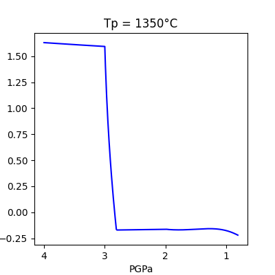
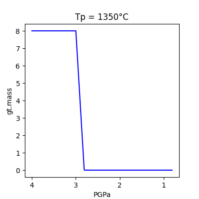
The easiest way to make a plot of a single run is to use the .plot() method. By default, the .plot() method creates a plot of logfO2_dFFM vs Pressure. To make other plots, indicate the x and y values as strings– any attribute of the ModelRun object is a valid input.

model_run.plot()

x= 'PGPa'
y= 'gt.mass'

model_run.plot(x,y)

5c. Making Data Tables

The easiest way to make a table of the main properties of a single run is to use the .get_data_table() method. You can save the results as a .xlsx by using .save_data_table() method. Be sure to download your output file to your local computer before exiting the Binder instance! Tables will not be saved! I also recommend changing the file name below if you have modified the tutorial code.

table = model_run.get_data_table()
# table     # (uncomment to display the table)

To add a column to the table, use the following notation

table['logfO2, dQFM'] = model_run.logfO2_dQFM
table['Fo#'] = model_run.olv.Fo_num
# table     # (uncomment to display the table)

To save the table as an Excel file, use the .save_data_table() method:

model_run.save_data_table('tutorial_output_table.xlsx')

If you have edited the data table (e.g., added columns), you’ll need to specify the new table for saving:

model_run.save_data_table('tutorial_output_table_edited.xlsx', data_table=table)